Advanced Lane Lines Detection
Python, OpenCV
Goals
The goals / steps of this project are the following:
- Compute the camera calibration matrix and distortion coefficients given a set of chessboard images.
- Apply a distortion correction to raw images.
- Use color transforms, gradients, etc., to create a thresholded binary image.
- Apply a perspective transform to rectify binary image (“birds-eye view”).
- Detect lane pixels and fit to find the lane boundary.
- Determine the curvature of the lane and vehicle position with respect to center.
- Warp the detected lane boundaries back onto the original image.
- Output visual display of the lane boundaries and numerical estimation of lane curvature and vehicle position.
Camera Calibration
The code for this step is contained in the first code cell of the IPython notebook located in “./project_submission.ipynb”
I start by preparing “object points”, which will be the (x, y, z) coordinates of the chessboard corners in the world. Here I am assuming the chessboard is fixed on the (x, y) plane at z=0, such that the object points are the same for each calibration image. Thus, objp is just a replicated array of coordinates, and objpoints will be appended with a copy of it every time I successfully detect all chessboard corners in a test image. imgpoints will be appended with the (x, y) pixel position of each of the corners in the image plane with each successful chessboard detection.
I then used the output objpoints and imgpoints to compute the camera calibration and distortion coefficients using the cv2.calibrateCamera() function. I applied this distortion correction to the test image using the cv2.undistort() function and obtained this result:

Pipeline (Single Image)
1. Applying cv2.undistort()
After obtaining the matrix for the camera distortion correction, I performed the cv2.undistort() function to each image so that I could show this step. The following is an illustration of what one of the test photographs looks like after I have applied the distortion correction:

2. Color Transforms, Gradients, and Thresholded Binary Image
First, I explored all possible color spaces to all images to isolate yellow lines and white lines. I took test5.jpg image as example because it has yellow lines, white lines, and different lighting conditions. Below are the original image and different color spaces.


Based on those images, I decided to compare several options for yellow and white lines detection.


I used B channel from LAB color space to isolate yellow line and S channel from HLS to isolate white color. After applying color thresholding for yellow color, I applied sobel x gradient to detect white lines. Combining them is the final step. Below is the visualitation of thresholding contribution after applying to all test images. Green color is to detect yellow line and blue color is to detect white line. The right side is combined binary threshold.

The code is titled “Thresholding” in the Jupyter notebook and the function is calc_thresh() which takes an image (img)as its input, as well as sobelx_thresh and color_thresh for threshold values.
3. Perspective Transformation
The code for my perspective transform includes a function called warp(), which appears in “Birds Eye View” section of the IPython notebook. The warp() function takes as inputs an image (img). I chose the hardcode the source and destination points in the following manner:
src = np.float32([(575,464),
                  (707,464),
                  (258,682),
                  (1049,682)])
dst = np.float32([(280,0),
                  (w-280,0),
                  (280,h),
                  (w-280,h)])
This resulted in the following source and destination points:
| Source | Destination |
|---|---|
| 575, 464 | 280, 0 |
| 707, 464 | 1000, 0 |
| 258, 682 | 280, 720 |
| 1049, 682 | 1000, 720 |
I verified that my perspective transform was working as expected by drawing the src and dst points onto a test image and its warped counterpart to verify that the lines appear parallel in the warped image.

4. Identifying Lane Lines Pixels
I created sliding_window_fit() and polyfit_tracking() to identify lane lines and fit second order polynomial for both left and right lines. It is put under “Detection using sliding window” and “Polyfit based on previous frame” section in Jupyter Notebook.
sliding_window_fit() takes a warped binary image as in input. It will calculate the histogram of the bottom second third of the image. Detection for yellow line in the left side quite good so that I decided to just get the local maxima from the left half of the image. However, for the right side, I put a sliding window to detect the base line which is put under “finding rightx base” section in the function. It calculates the number of detected pixel in y direction within the window. It saves the value in a temporary array and return back the index of maximum value. This is more robust compared to finding local maxima which may lead to detect noise. The function then identifies nine windows from which to identify lane pixels, each one centered on the midpoint of the pixels from the window below. This effectively “follows” the lane lines up to the top of the binary image. I collect pixels that are inside the window and use np.polyfit() to get a second order polynomial equation.

Once I get the result from the previous frame, I applied polyfit_tracking() which takes an binary warped image as an input, as well as previous fit for left and right side. This function will search nonzero pixel within 80 margin of each polynomial fit. It will speed up the process because I don’t need to blindly search from beginning.
5. Calculating Radius of Curvature and Position of the Vehicle with Respect to Center
The curcature measurement is written under “Determine the curvature of the lane” section in Jupyter Notebook
The radius of curvature is based upon this website and calculated in the code cell titled “Radius of Curvature and Distance from Lane Center Calculation” using this line of code (altered for clarity):
curve_radius = ((1 + (2*fit[0]*y_0*y_meters_per_pixel + fit[1])**2)**1.5) / np.absolute(2*fit[0])
y_meters_per_pixel is determined by eyeballing the image. Below are the constants I used for calculation.
ym_per_pix = 30/720
xm_per_pix = 3.7/700
calc_curvature also calculates the position of the vehicle with respect to center. Assuming the camera is in the middle of the vehicle, the position can be estimated by substracting car position, which is binary_warped.shape[1]/2, and lane centre position, (r_fit_x + l_fit_x)/2. The result of the substraction will be scaled by xm_per_pixel to get meter as the unit.
6. Inverse Persepective Transformation
This phase is implemented in the function draw lane() in the section "Warp the detected lane borders back onto the original image". This function requires the following inputs: original img, binary img, l fit, r fit, Minv.
Minv includes an inverse matrix for transforming a twisted image back to its original state. Overlaying it with cv2.addWeighted() will make it appear good.
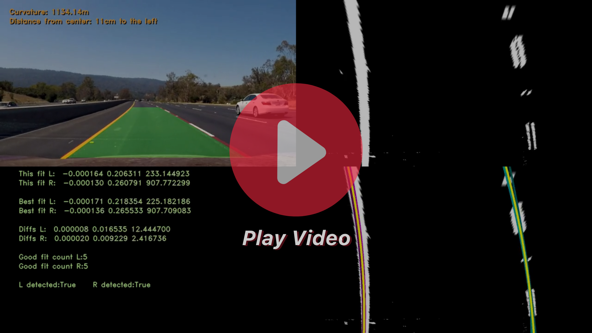
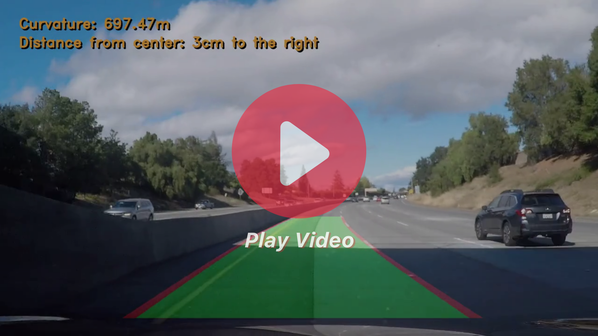
After generating the map, I used the put curvature() method to add the curvature and vehicle position information to the upper left of the image.
Here’s an example of my output from a test image:

Result
Possible Improvements to the Current Pipeline
The issue is that my pipeline isn’t built to withstand harsh lighting, shadows, and bumpy roads. I believe that employing deep learning for image segmentation is a better method. We can then get the lines and utilize them to determine the lane.
I also doubt using a bird’s eye view is the best approach. I’d appreciate it if you could share any relevant articles or studies with me.